Scale invariance and the concept of universality class
The one-dimensional and the two-dimensional random walks can demonstrate two very important concepts in statistical mechanics. One is scale invariance; the other is the universality class.
Scale invariance
Suppose we have \(N_1\) to be a big enough number. According to our derivation, the r.m.s. for the magnitude of the displacement vector is \(\sqrt{N_1}\). When we have \(N_2\) which is also large, we will similarly have the r.m.s to be \(\sqrt{N_2}\). This is an example of scale invariance. The statistical property of the case with \(N_1\) steps and \(N_2\) steps is identical in the sense that the r.m.s both have the square root dependence of the total step number. It might look trivial in this example. However, it is possible to have scale invariance emerging in non-trivial systems.
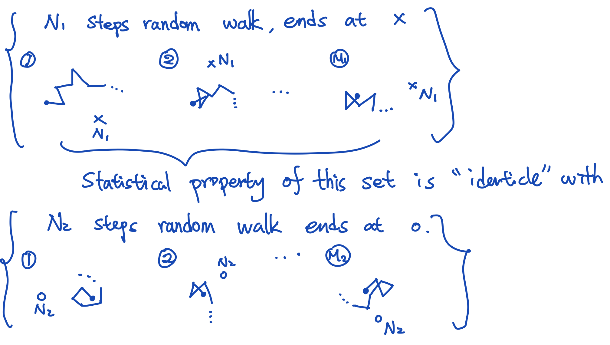
Fig. 6 Concept of scale invariance.
The concept of universality class
The one-dimensional and the two-dimensional random walks are different. However, we observe the r.m.s. for the magnitude of the displacement vector share the same functional form, \(\sqrt{N}\) behavior. Therefore, it is very likely that the two models are related to each other somehow. This is an example of the idea of universality classes. The term just means that various systems could share similar behavior because the key mechanism behind the two systems is identical. In this example, the key mechanism for the two examples is: the steps are random in their orientation. Since the model is simple, we can understand the physics explicitly. Even though the two systems are in different dimensions, the fact that \(\langle X_{s-1}l_s\rangle=0\) (in 1D) and \(\langle \textbf{X}_{s-1}\cdot\textbf{l}_s\rangle=0\) (in 2D) and the unit step size guarantee the \(\sqrt{N}\) behavior of the r.m.s. So the detail of whether it is one-dimensional or two-dimensional is irrelevant.
When we say some of the microscopic detail is irrelevant, it also means some of the “details” are relevant. A natural question to ask is: in these simple examples, how to change the \(\sqrt{N}\) behavior of the r.m.s.? We can go back to our derivation and see that the unit step size condition helps us to get to the \(\sqrt{N}\) result explicitly. Can we relax that condition and modify our result? Maybe the drunk guy is too drunk, so he cannot maintain the step size anymore. How would that change our conclusion?
We will introduce an example of the relevant couplings using the polymer system in the next section first. After that, we will discuss the issue of random step size and derive the macroscopic description or the effective theory of our system. We will see our microscopic model leads to the diffusion equation. By solving the diffusion equation, we will find the similar \(\sqrt{N}\) behavior. That suggests the fixed step size condition is irrelevant for this universality class.
The polymer and the random walks
How is the idea of random walks related to some of the real-world systems? One of the interesting examples is the radius of a polymer. A polymer is a long molecule formed by small units(monomers). For example, DNA, proteins, and rubbers are all formed by polymers. Those monomers interact with each other, so the polymers will fold themselves in a particular way to lower their energy. However, when the temperature is high enough, the monomers will fluctuate more, and the polymer will look like a chain of linked sausage fluctuating in the environment. Assuming we have only one type of monomer, when the temperature is high enough, the angle between two sausage links will be a random number. Since the monomer size is fixed, the polymer will look like a drunkard’s walk model where the number of monomers for each polymer molecule corresponds to the number of steps in the drunkard’s walk problem.
However, there is a relevant difference between the polymer system and the drunkards walk problem. The monomers cannot pass each other as if they are phantom monomers. That means the corresponding random walk path has a constraint that the path cannot cross each other. That is the so-called self-avoiding random path. This tiny difference actually can modify the \(\sqrt{N}\) behavior of the r.m.s. In two-dimensional systems, we have \(\sigma_{\textbf{X}_N}\propto N^{\nu}\). For the random walk model, we have \(\nu=\frac{1}{2}\). For the self-avoiding walk, we have \(\nu=\frac{3}{4}\). This is an example of the relevant couplings.
Here, we just use simple examples to demonstrate the idea of scale invariance and the universality classes. Is there a theoretical framework that can understand such behavior in a systematic way? Can we find a way to identify relevant couplings from irrelevant couplings? Those are interesting sharp questions to be asked, and they are discussed in the theory of renormalization group. It is an important concept to understand the interacting theories using statistical mechanics. We might discuss this concept later this semester or in Statistical mechanics (II).